
1.概要
単純パーセプトロンは、最も基本的な形式のニューラルネットワークで、1つのニューロンから構成されます。入力ベクトルと重みベクトルの内積にバイアスを加え、その結果を活性化関数(しきい値関数)によって出力します。線形分離可能な問題に対して適していますが、非線形問題には対応できません。
すなわち、入力データが線形平面で2つのクラスに分けられる場合にのみ分類が可能となり、非線形な問題や複雑なクラスの境界線を持つ問題には対応できません。多クラス分類問題に対応するには、複数の単純パーセプトロンを組み合わせたり、他の手法(例えば多クラスロジスティック回帰や多層パーセプトロン)を使用する必要があります。
雑なモデルや手法を検討する必要があります。
2.パーセプトロンの構造と動作
パーセプトロンは、ニューラルネットワークの最も基本的な単位であり、単層の線形分類器です。1950年代から1960年代にかけて、フランク・ローゼンブラットによって考案されました。パーセプトロンは、与えられた入力データを2つのクラスに分類するために使用されます。
(1)パーセプトロンの構造と動作
パーセプトロンの基本的な構造は次の通りです。
①入力層
特徴量ベクトルx=[x1,x2,・・・,xn]を入力します。各特徴量は重み付けされます。
②重みとバイアス
各入力特徴量には対応する重み w=[w1,w2,・・・,wn]があります。
バイアスb は、入力に対する追加の定数項です。
③線形結合
入力特徴量と重みのドット積にバイアスを加えて、線形出力zを計算します。
z = w・x+b ”・”はベクトル積
④活性化関数
線形出力z に対して活性化関数を適用し、最終的な出力yを得ます。
パーセプトロンでは、ステップ関数(Heavisideステップ関数)が一般的に使用されます。
(2)パーセプトロンの学習
パーセプトロンは、誤差修正アルゴリズム(パーセプトロン学習アルゴリズム)を使用して重みとバイアスを更新します。学習の手順は以下の通りです。
①初期化:
重みベクトルw とバイアスb を小さなランダムな値で初期化します。
②各トレーニングデータポイントの処理:
各トレーニングデータ(x,y_true)に対して、以下を行います
・線形出力zを計算します
z = w・x+b ”・”はベクトル積
・活性化関数を適用して予測ypredを得ます
・誤差を計算します
error=ytrue-ypred
・重みとバイアスを更新します
③エポック
上記の処理を全てのトレーニングデータに対して行い、これを複数回(エポック)繰り返します。
3.単純パーセプトロンのサンプル
import numpy as np

class SimplePerceptron:
    def __init__(self, num_features, learning_rate=0.1, epochs=4):
        self.num_features = num_features
        self.learning_rate = learning_rate
        self.epochs = epochs
        self.weights = np.zeros(num_features)
        self.bias = 0.0

    def predict(self, x): #x:トレーニングデータ、又はテストデータ(特徴量ベクトル)
        linear_output = np.dot(self.weights, x) + self.bias #線形結合
        prediction = 1 if linear_output > 0 else 0 #活性化関数(ステップ関数)
        return prediction #予測結果を返す

    def train(self, X_train, y_train):
        for epoch in range(self.epochs):
            for x, y_true in zip(X_train, y_train):
                y_pred = self.predict(x)#予測結果
                error = y_true - y_pred #誤差の計算
                self.weights += self.learning_rate * error * x #重み更新(w←w+η(学習率)⋅error⋅x)
                self.bias += self.learning_rate * error #バイアス更新(b←b+η(学習率)⋅error)
                print("epoch:",epoch,"self.weights:",self.weights,"self.bias:",self.bias)

    def evaluate(self, X_test, y_test):
        print("*** evaluate ***")
        correct = 0
        for x, y_true in zip(X_test, y_test):
            y_pred = self.predict(x)
            if y_pred == y_true:
                correct += 1
        accuracy = correct / len(y_test)
        return accuracy

# Example usage:
if __name__ == "__main__":
    # Example dataset
    X_train = np.array([[0.9, 0.8], [0.7, 0], [0.3, 0.5], [0, 0]])
    y_train = np.array([1, 1, 0, 0])  # Binary labels (1 or 0)

    # Create and train the Simple Perceptron
    perceptron = SimplePerceptron(num_features=2)
    perceptron.train(X_train, y_train)

    # Example evaluation
    X_test = np.array([[0.6, 0.6], [0.7, 0.3], [0.2, 0.4], [0.6, 0.2]])
    y_test = np.array([1, 1, 0, 0])
    accuracy = perceptron.evaluate(X_test, y_test)

    print(f"Accuracy: {accuracy}")
#トレーニングデータ
#X_train = np.array([[0.9, 0.8], [0.7, 0], [0.3, #0.5], [0, 0]])
#y_train = np.array([1, 1, 0, 0])
#テストデータ
#X_test = np.array([[0.6, 0.6], [0.7, 0.3], [0.2, #0.4], [0.6, 0.2]])
#y_test = np.array([1, 1, 0, 0])
#実行結果
#epoch: 1 self.weights: [ 0.03 -0.02] self.bias: -0.1
#epoch: 2 self.weights: [0.09 0.01] self.bias: -0.1
#epoch: 3 self.weights: [0.15 0.04] self.bias: -0.1
#Accuracy: 1.0 トレーニングデータ、テストデータ、及びepoch毎の実行結果weights、biasの線形出力をグラフに表示します。
ここで、トレーニングデータのラベル0:青×、ラベル1:青○、テストデータのラベル0:赤×、ラベル1:赤○とします。
import matplotlib.pyplot as plt
import numpy as np

# データ
data_circle = [[0.9, 0.8], [0.7, 0]]
data_cross = [[0.3, 0.5], [0, 0]]
test_circle = [[0.6, 0.6], [0.7, 0.3]]
test_cross = [[0.2, 0.4], [0.6, 0.2]]

# データをX軸とY軸に分割
x_circle, y_circle = zip(*data_circle)
x_cross, y_cross = zip(*data_cross)
xt_circle, yt_circle = zip(*test_circle)
xt_cross, yt_cross = zip(*test_cross)

# プロット
plt.figure(figsize=(8, 6))
plt.scatter(x_circle, y_circle, marker='o', color='b', label='label:1')
plt.scatter(x_cross, y_cross, marker='x', color='b', label='label:0')
plt.scatter(xt_circle, yt_circle, marker='o', color='r', label='label:1')
plt.scatter(xt_cross, yt_cross, marker='x', color='r', label='label:0')

# 直線のプロット
x_line = np.linspace(-0.1, 1, 400)  # x範囲を設定
y_line1 = -0.15 * x_line / 0.04 + 0.1 / 0.04
y_line2 = -0.03 * x_line / (-0.02) + 0.1 / (-0.02)
y_line3 = -0.09 * x_line / 0.01 + 0.1 / 0.01
plt.plot(x_line, y_line1, color='g', label='epoch:3 y=-0.15*x/0.04+0.1/0.04')
plt.plot(x_line, y_line2, color='y', label='epoch:1 y=-0.03*x/(-0.02)+0.1/(-0.02)')
plt.plot(x_line, y_line3, color='m', label='epoch:2 y=-0.09*x/0.01+0.1/0.01')


plt.title('SimplePerceptron blue:train red:test')
plt.xlabel('X')
plt.ylabel('Y')
plt.legend()
plt.grid(True)
plt.show()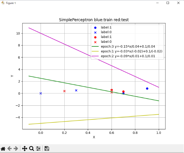
4.プログラムの解説
(1)SimplePerceptron クラスの初期化
def __init__(self, num_features, learning_rate=0.1, epochs=4):
        self.num_features = num_features
        self.learning_rate = learning_rate
        self.epochs = epochs
        self.weights = np.zeros(num_features)
        self.bias = 0.0
・特徴量の数 num_featuresを設定し、重みベクトルの初期化を行います。
self.num_features: 2
self.weights: [0. 0.]
・学習率 learning_rate、エポック数 epochs を設定します。
(2)predict メソッド(予測値を算出)
def predict(self, x): #x:トレーニングデータ、又はテストデータ(特徴量ベクトル)
        linear_output = np.dot(self.weights, x) + self.bias #線形結合
        prediction = 1 if linear_output > 0 else 0 #活性化関数(ステップ関数)
        return prediction #予測結果を返す
入力ベクトル(特徴量) x を用いて予測を行います。線形結合の結果を活性化関数として使い、閾値に基づいて予測を二値化します。
・linear_output = np.dot(self.weights, x) + self.bias
重みと特徴量のベクトル積にバイアス値を加算(線形結合)
・prediction = 1 if linear_output > 0 else 0
三項演算子を使用しており、linear_output が 0 より大きい場合は 1 を、そうでない場合は 0 を prediction に代入します。
(3)train()メソッド(重み、バイアスの更新)
def train(self, X_train, y_train):
        for epoch in range(self.epochs):
            for x, y_true in zip(X_train, y_train):
                y_pred = self.predict(x)#予測結果
                error = y_true - y_pred #誤差の計算
                self.weights += self.learning_rate * error * x #重み更新(w←w+η(学習率)⋅error⋅x)
                self.bias += self.learning_rate * error #バイアス更新(b←b+η(学習率)⋅error)
                print("epoch:",epoch,"self.weights:",self.weights,"self.bias:",self.bias)
・与えられた訓練データ X_train(特徴量ベクトル) と y_train(ラベル値) を用いてパーセプトロンを学習します。各訓練データに対して予測を行い、誤差を計算し重みとバイアスを更新します。これをエポック数繰り返します。
・for x, y_true in zip(X_train, y_train):
X_train, y_train リストの要素を取り出す
(4)evaluate()メソッド(評価)
def evaluate(self, X_test, y_test):
        print("*** evaluate ***")
        correct = 0
        for x, y_true in zip(X_test, y_test):
            y_pred = self.predict(x)
            if y_pred == y_true:
                correct += 1
        accuracy = correct / len(y_test)
        return accuracy
・train()メソッドで算出した、weights(重みベクトル)、bias(バイアス値)を使って、予測値を算出し、ラベルの値と一致するか否かの評価を行う。
(5)main
# Example usage:
if __name__ == "__main__":
    # Example dataset
    X_train = np.array([[0.9, 0.8], [0.7, 0], [0.3, 0.5], [0, 0]])
    y_train = np.array([1, 1, 0, 0])  # Binary labels (1 or 0)

    # Create and train the Simple Perceptron
    perceptron = SimplePerceptron(num_features=2)
    perceptron.train(X_train, y_train)

    # Example evaluation
    X_test = np.array([[0.6, 0.6], [0.7, 0.3], [0.2, 0.4], [0.6, 0.2]])
    y_test = np.array([1, 1, 0, 0])
    accuracy = perceptron.evaluate(X_test, y_test)

    print(f"Accuracy: {accuracy}")
・if name == “main“
スクリプトが直接実行されたときにのみ、実行するための条件文
・np.array()でndarrayオブジェクトに変換する
・SimplePerceptron(num_features=2)でインスタンスを生成
・train()メソッドで重みベクトル、バイアス値の更新
・evaluate()で評価する
以上